Matlab Bindings for HybMesh

Usage

Matlab (Octave) bindings contain set of source *.m files (one for each class) and a pair of shared libraries core_hmconnection_oct.oct, core_hmconnection_matlab for Octave and Matlab communication respectively. The most convenient way to deal with all that mess is to use addpath directive to include the whole bindings directory. After that the Hybmesh class will be available. To set directory containing hybmesh executable (if it differs from the default) use static Hybmesh.hybmesh_exec_path() method.

Like Python interface, matlab wrapper doesn’t provide special point classes. Instead a raw vector with 2 or 3 entries should be used to pass a point to a function. When point list of size n is needed use nx2 or nx3 matrix. When list of geometrical objects is needed use cell arrays. In the following example two contours are created by passing a list of points and then they are connected by a method taking cell array of contour objects as argument:

hm = Hybmesh();
c25 = hm.create_contour([0, 0; 1, 0; 2, 0]);
c26 = hm.create_contour([2, 0.1; 3, 0.1; 4, 1]);
c27 = hm.connect_subcontours({c25, c26}, []);

nan value is used instead of Python None where not-defined object should be passed.

As it was mentioned above there are no special exception classes in Matlab bindings (since they are not supported by Octave). Instead simple error() calls are used which could also be handled in try...catch...end blocks.

Warning

Native Matlab indexing starts from one. However Hybmesh operates with zero based indices. So all hybmesh wrapper functions which require indices as arguments or return set of indices of any kind use C-style indexing.

Some wrapper functions ending arguments could be omitted in order to use their default values. Such arguments along with their default values are specified in function documentation. For example this is Hybmesh method for building rectangular grid as it is defined in Hybmesh.m wrapper file

function ret=add_unf_rect_grid(self, p0, p1, nx, ny, bnd)
% ADD_UNF_RECT_GRID
% Builds rectangular grid.
%   p0: 2d point as [x, y];
%   p1: 2d point as [x, y];
%   nx: int;
%   ny: int;
%   bnd: row vector of int. DEFAULT is [0, 0, 0, 0];
%   ----
%   returns: GRID2D;
%
% See details in hybmeshpack.hmscript.add_unf_rect_grid().
    if (nargin < 6)
        bnd = [0, 0, 0, 0];
    end
    ....

Here the first argument is used to address Hybmesh instance. The function by itself takes 5 parameters, but also could be called with only 4. In the latter case default bnd = [0, 0, 0, 0] will be used.

Hybmesh is a handle class which has a destructor delete method. Until this method is called hybmesh background executable will not stop working. Matlab calls it implicitly when an instance of Hybmesh gets out of context. However if this instance presents in the global scope, it is recommended to destroy it manually either by invocation of delete method or using clear directive.

For detailed description of all methods consult the Python binding functions reference and embedded documentation of wrapper *.m files.

Helloworld Example

After successful hybmesh installation create the following file replacing path at the first line if needed and run it as a usual Matlab/Octave script

hmtest.m

addpath('C:/Program Files/Hybmesh/include/m');

hm = Hybmesh();
g = hm.add_unf_rect_grid([0, 0], [1, 1], 2, 2);
d = g.dims();
fprintf('number of cells: %i\n', d(3));
clear hm;

Introductory Example

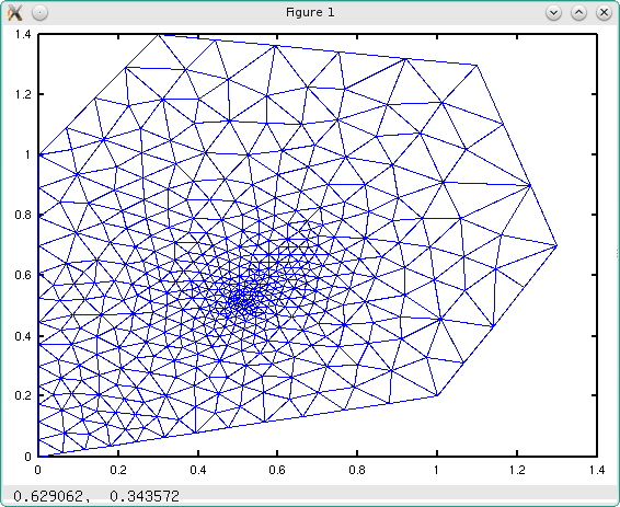
In this example a simple unstructured triangle grid in custom polygon is built and displayed. Grid step sizes are defined by reference point boundary partition and two embedded point conditions. The unstructured triangulation is performed by internal call of corresponding GMSH method.

% add directory where Hybmesh.m is located
addpath('../../../../build/bindings/m');
% initialize hybmesh object
hm = Hybmesh();

% set verbose stdout output
hm.stdout_verbosity(3);

% define set of points bounding triangulated area
% first equals last for closed contours.
points = [0.0, 0.0;
    0.5, 0.1;
    1.0, 0.2;
    1.3, 0.7;
    1.1, 1.3;
    0.3, 1.4;
    0.0, 1.0;
    0.0, 0.0];

% create a bounding contour
cont = hm.create_contour(points);

% perform contour parition using reference points:
% - at point closest to [0, 0] recommended size is 0.05,
% - at point closest to [1, 1] recommended size is 0.2.
domain = hm.partition_contour_ref_points(cont, [0.05, 0.2], [0, 0; 1, 1]);

% add two inner points which should present in result
inner_points = [0.5, 0.5; 0.7, 0.7];

% triangulate domain with two additional inner points
% with recommended step sizes 0.01, 0.03 respectively.
grid = hm.triangulate_domain(domain, [], [0.01, 0.03], inner_points);

% get grid vertices as plain [x0, y0, x1, y1, ....] array
pts = grid.raw_vertices();

% get cell-vertices table as plain array of vertex indicies where
% each three represent a triangle. Indexing starts with zero.
tris = grid.raw_tab('cell_vert');

% modify grid data to be able to plot it using triplot function:
% 1. slice pts array into separate x and y arrays
x=pts(1:2:end);
y=pts(2:2:end);
% 2. reshape tris into 2D matrix and add unity to fit native indexing
tris = reshape(tris, 3, [])' + 1;

% explicitly free hybmesh handle
clear hm;

% plot data
triplot(tris, x, y);