Grid Prototypes¶

Rectangle Grid¶

Builds a rectangular structured grid with given partition along x and y axis. User can define partition as number of equidistant segments, as a constant step or explicitly define partition by passing increasing array of respective coordinates.

Python interface function: add_unf_rect_grid().

Radial Grid¶

Builds structured radial grid. Central element could be triangulated or left as a regular n-side polygon. Radial and arch partition could be defined by number of steps, step size or explicitly. Refinement of radius partition could also be applied.

Python interface function: add_unf_circ_grid().

Ring Grid¶

Builds structured radial grid in a ring area. Refinement of radius partition could also be applied.

Python interface function: add_unf_ring_grid().

Triangle Grid¶

Builds structured grid in a triangle domain given by three points. Resulting grid will contain quadrangle cells everywhere except area near one of the edges where triangle cells will be built.

Python interface function: add_triangle_grid().

Hexagonal grid¶

Builds a structured regular hexagonal mesh in hexagonal or rectangular area (see figure below).

Regular hexagonal mesh in hexagonal and rectangle areas

User defines hexagonal cell radius and area size. In case of hexagonal area user passes center of the area and its radius. In case of rectangular area two corner points of rectangle should be assigned. The algorithm of sizes treatment is shown in the figure below.

Regular hexagonal mesh area sizes

A special strict option defines whether program should stretch a grid to inscribe it into a user area. Using nomenclature given in the above picture this would guarantee $R^r = R^u$ for hexagonal area and $H_x^r = H_x^u$ , $H_y^r = H_y^u$ for rectangular area. In the latter case this would most likely make grid cells non-regular (slightly stretched in x or y direction). But this procedure could be a handy tool to prepare this grid for clipping with user rectangle. With such stretch all boundary cells will be cut through their middle axis (see figure below).

Clipped hexagonal mesh built in rectangle area with different strict settings.

Python interface function: add_unf_hex_grid().

Square in Circle¶

This creates a quadrangular cell grid in a circular area in such a way that the resulting grid contains uniform square grid in the center of defined area which is extended by a ring-like grid towards the outer circular boundary as it is shown in the figure below.

Square in circle grids built with different options

Geometry of the circular area is defined by the center point and radius. Partition is calculated using the approximate size of outer boundary step passed by user. Since the grid in the ring part of the area is built in a $\pi/4$ sector, resulting number of steps along outer boundary will be divisible by 8.

Size of the inner square is defined by a parameter a equals the ratio of circle radius to square side length. Its default value is unity and, apparently, it can not be greater than $\sqrt2$ .

Additionally user can define refinement coefficient for the ring grid in a radius direction. This coefficient approximately equals the ratio of the first step in a radial direction at $\pi/4$ to the outer boundary step. Values less than unity lead to a refinement towards the outer boundary.

Four algorithms of building ring part of the grid are implemented:

Linear algorithm. Radial lines are created by linear connection of corresponding points on outer an inner segments. Then these lines are divided keeping constant reference weights of each step.
Laplace algorithm. An algebraic mapping from a uniform square grid to the sector area is built in such a way that each boundary sector vertex be mapped to a uniform square boundary vertex.
Orthogonal with uniform rectangle grid. An orthogonal mapping from a rectangle to the sector area is built. Arc grid lines are built starting from the predefined vertices of the shortest radius line. Radial grid lines start from the predefined square sides vertices.
Orthogonal with uniform circular grid. The same as the previous but radial lines start from outer circle vertices.

The first, second and third algorithms give uniform grid within inner square; the first, second and forth - uniform outer circle partition. Only last two algorithms build an orthogonal grid.

Python interface function: add_circ_rect_grid().

Custom Rectangle Grid¶

Builds a structured quadrangle grid within an area bounded by four curvilinear sides.

For the sake of clarity let us denote four basic contours as left, bottom, right, and top. This nomenclature is conventional, it doesn’t reflect real geometrical position but only the fact that horizontal grid lines will connect vertices from left and right contour and vertical lines - vertices from bottom and top contours. Boundary vertices of resulting grid will equal input contour vertices, hence number of cells in resulting grid is defined by the partition of passed contour.

There is no need to exactly connect contours before passing ‘em to grid constructor. The direction of passed contours also doesn’t matter. The program will try to translate and stretch contours to build a closed domain with minimum translation distance possible. The order of input contour transformations is:

place the left contour as it is;
connect the bottom contour with the left contour bottom point;
connect the top contour with the left contour top point;
connect the right contour with the bottom contour right point;
stretch the right contour so its upper point fits top contour right point.

As a result of these modifications

for the contour passed as left both position and shape are preserved,
for the top and bottom contours shape is preserved,
for the right both position and shape could be changed.

The definition of right and/or top contours could be omitted. If so then the right/top contour will be built by parallel translation of the left/bottom one. The resulting domains built by different input contours are shown in figure below.

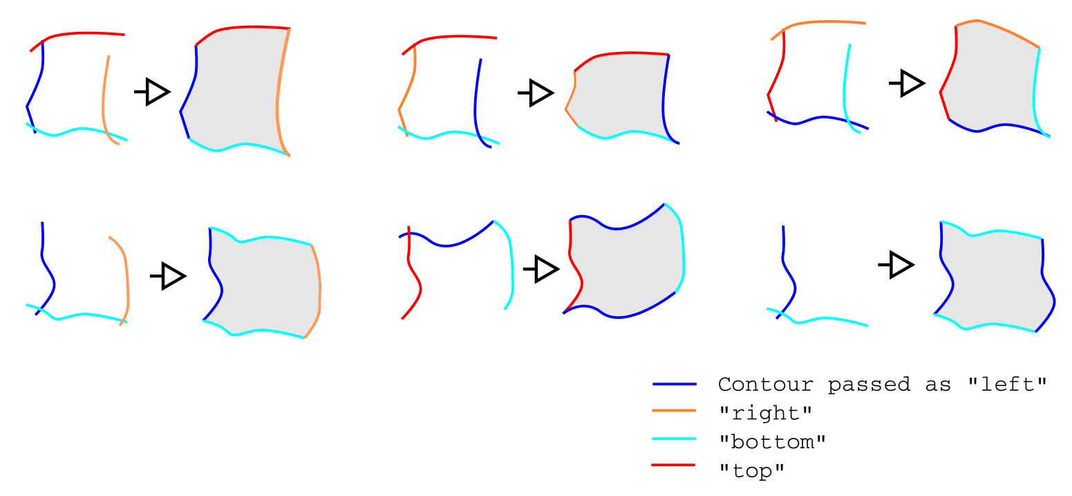
Assembling closed domain based on not connected base contours

Boundary features of resulting grid are inherited from the boundary features of input contours.

Six algorithms of building internal grid nodes are implemented. Examples of grids built using different algorithms is shown in figure below.

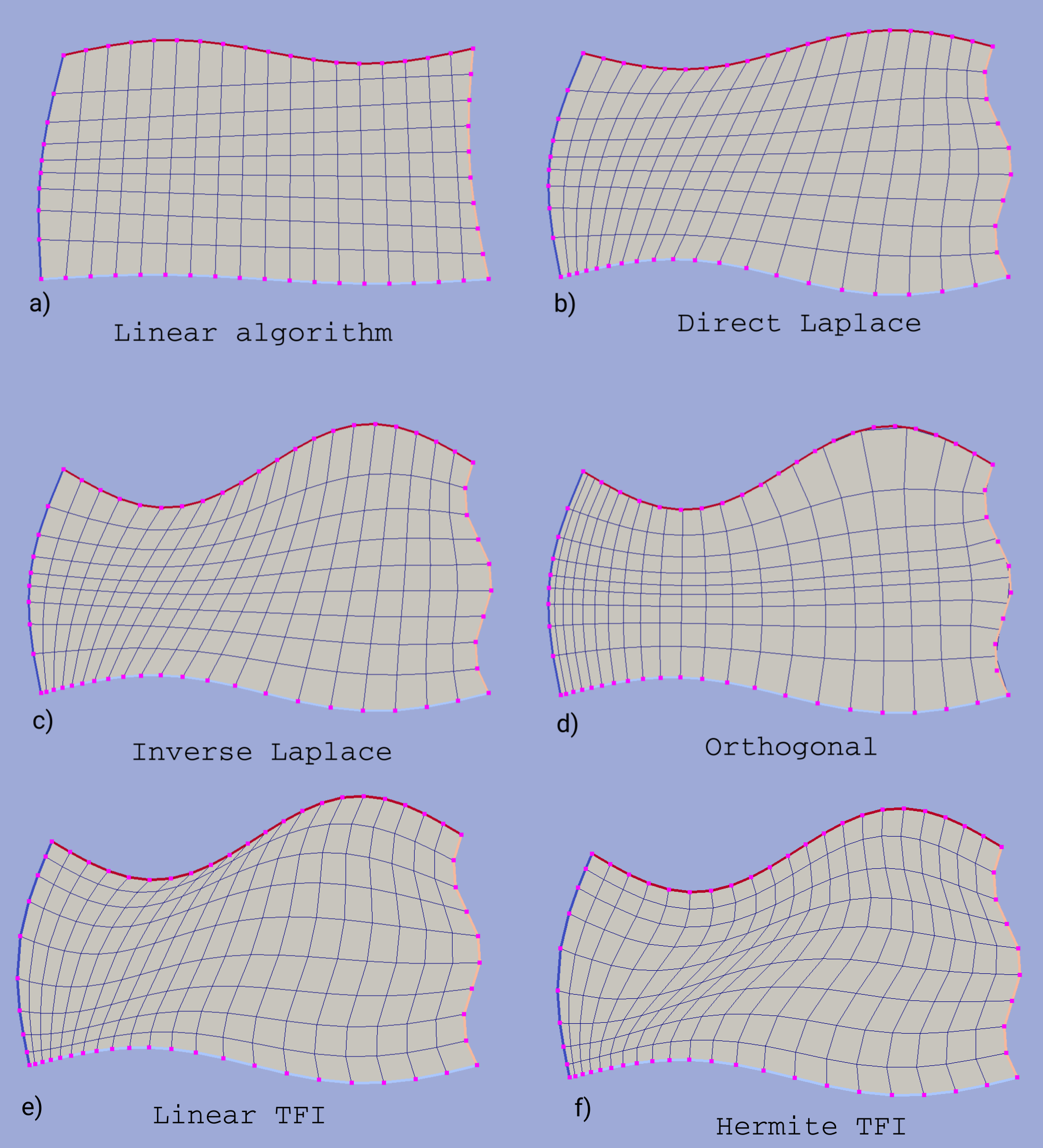
Custom rectangular grids built using different algorithms. Passed contours vertices are shown by magenta marks.

Linear algorithm. Corresponding vertices from opposite contours are connected by straight lines and grid cells are built on intersection points. This is the fastest algorithm although it doesn’t provide smoothing near the curvilinear edges, hence it should be used only if input contours are straight lines.

Linear transfinite interpolation (TFI). An algebraic mapping which uses boolean sum of linear weighted transformations built between opposite contours.

Hermite transfinite interpolation. The same as previous but weighted transformations between opposite contours are built using cubic polynomials providing perpendicular grid lines. For this algorithm user has to define perpendicularity coefficients for each given contour. The greater this coefficient the further the influence of corresponding contour propagates inward the domain. The effect of this coefficient is illustrated in figure below. Note that the resulting grid will not be orthogonal but only close to it.

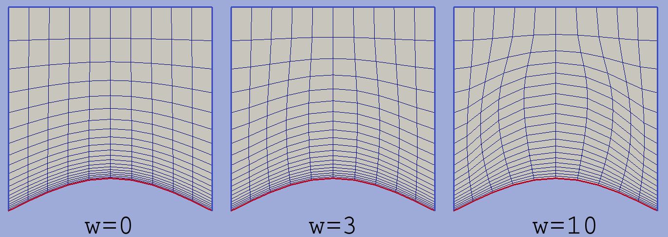
Hermite interpolation with different perpendicularity coefficients w for bottom boundary. Coefficients for left, right and top segments were set to zero.

Direct/Inverse Laplace algorithm. Mapping from unit square to input domain is built using the direct or inverse laplace algorithm. To build a grid line (horizontal or vertical) first its start points are defined in physical domain, then these points are translated into unit domain where they are connected by a straight line which is finally mapped back to the physical domain. Explanation of algebraic mapping building, difference between direct and inverse algorithms and their limitations can be found in Algorithms. Since unit square is used as a base domain then the inverse algorithm always gives valid results whereas the direct may fail due to grid self-intersections.

Orthogonal algorithm. This method builds an orthogonal mapping from input domain to the unit square based on a solution of Laplace equation with mixed boundary conditions. To build a vertical line first a start point in physical area is defined by a vertex of the bottom contour. Then this point is translated into the unit domain from which a strictly vertical line is built and mapped back into the physical area. Horizontal grid lines built in the similar way starting from vertices of the left contour. The resulting grid is guaranteed to be orthogonal disregarding the grid edges straightening.

Linear, tfi and Laplace algorithms demand equal partition of opposite contours. Orthogonal algorithm completely ignores partition of right and top contours.

Python interface function: add_custom_rect_grid().

Boundary Grids¶

TODO

Grid Prototypes¶

Rectangle Grid¶

Radial Grid¶

Ring Grid¶

Triangle Grid¶

Hexagonal grid¶

Square in Circle¶

Custom Rectangle Grid¶

Boundary Grids¶

Table Of Contents

Previous topic

Next topic

This Page