Example 6
In the present example a grid for a typical oil reservoir simulation problem will be built. The modeling area is a square which contains three well sites and a fracture contour (or horizontal well contour) (see fig. 1 below). Flow patterns of such problems provide very large fluid velocity gradients near wells and fractures hence it is a common practice to build grids with substantial refinement towards well and fracture locations.
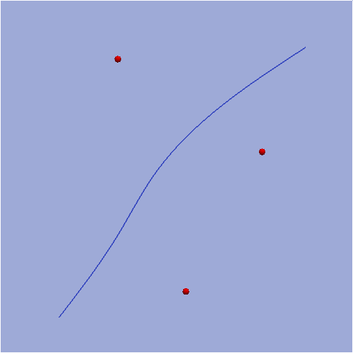
fig. 1
Required grid depends on a numerical method. First lets assume we build a grid which will be used in a linear finite element solver. Hence we need a grid which contains only triangle/quadrangle cells, well locations are its vertices and fracture contour segments coincide with its edges.
The simplest straightforward approach is to use unstructured conditional triangulation. Hybmesh script for that algorithm contains three lines (operations):
- fracture contour partition;
- domain contour partition;
- conditional domain triangulation.
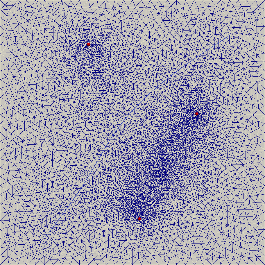
fig. 2
The resulting grid (depicted in fig. 2) has at least two evident flaws. First the refinement from the upper well towards the upper domain segment is very coarse. It happened because we have explicitly defined partition of domain boundary without taking well locations into account. Another problem is that the region between two lower wells is meshed too fine because even far away from their sites these wells remain the closest cell size detection sources.
To overcome those flaws we will use conditional 1D partition of domain boundary and place a supplementary cell size condition between two lower wells. Furthermore we will use recombine algorithm to turn our triangle mesh to a mesh containing mostly quadrangle cells. The result is shown in figure 3.
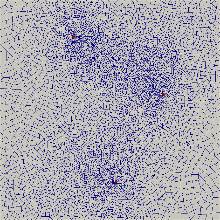
fig. 3
Despite we’ve defined mesh refinement in the regions of high fluid flow velocities the numerical solution could still be imperfect because of usage of unstructured grids near well bores. We can increase solution accuracy by building a radial grids around wells which are known to provide better solution for radial symmetric flows thus using locally structured approach to grid generation. So we build three radial grid prototypes to treat well zones, stripe grid prototype in a fracture zone and impose them onto a regular quadrangle substrate grid. Result is shown in figure 4.
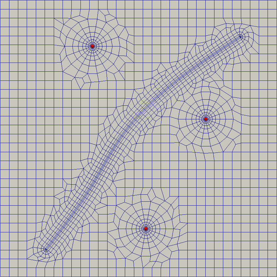
fig. 4
Now we’ll illustrate usage of Hybmesh for finite volume grid generation. Such grids can contain arbitrary cells (regular polygons are preferred). Well sites should lie in the centers of cells. Location of fracture contour depends on numerical algorithm. We will place it to the cell centers too (as it would be if this is a horizontal well contour).
As before we can use simple straightforward approach by execution of conditional unstructured griding routine with perpendicular bisector cells (figure 5) or apply locally structured approach (figure 6). We also can utilize any of those 2D grids to build 3D ones using simple extrusion algorithm (figure 7).
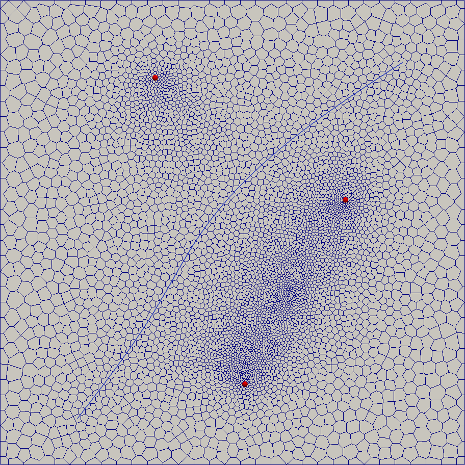
fig. 5
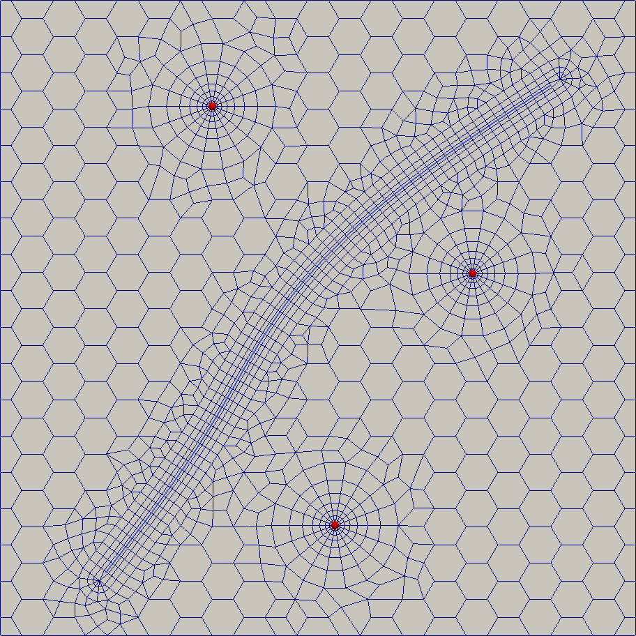
fig. 6
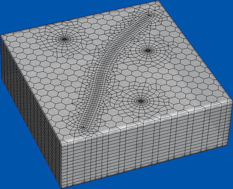
fig. 7
from hybmeshpack import hmscript as hm
# This script was created for hybmesh 0.4.5.
# If running version of hybmesh is not compatible with this version
# an exception will be raised at this line.
hm.check_compatibility("0.4.5", 2)

# ====================== Input data
# define wells coordinates
w1 = [100, 250]
w2 = [223, 171]
w3 = [158, 52]

# area and fracture coordinates
area_pts = [0, 0], [300, 300]
crack_pts = [50, 30], [100, 100], [130, 150], [260, 260]

# meshing options
w_size = 1      # grid cell size near well zones
dom_size = 10   # grid cell size in outer domain
crack_size = 5  # grid cell size along fracture

# building geometric entities
# (see fig.1)
area = hm.add_rect_contour(*area_pts)
crack = hm.create_spline_contour(list(crack_pts))


# ======================= FEM mesh
# 1. Unstructured triangulation
# make 1D partition of geometry using recommended sizes
pcrack = hm.partition_contour(crack, 'const', crack_size)
parea = hm.partition_contour(area, 'const', dom_size)

# build unstructured conditional triangulation of the domain so
# that all well points and fracture edges be preserved as grid entities
# and cell sizes near well be equal to w_size
# (see fig.2)
fin2 = hm.triangulate_domain(
    parea, [pcrack], [w_size, w1, w_size, w2, w_size, w3])

# 2. Quadrangulation with boundaries refinement
# make 1D partition of a crack keeping in mind mesh refinement
# near well sites.
pcrack = hm.matched_partition(
    crack, crack_size, 80, [], [w_size, w1, w_size, w2, w_size, w3])

# make 1D partition of an outer area keeping in mind mesh sizes
# at fracture and well sites
parea = hm.matched_partition(
    area, dom_size, 80, [pcrack], [w_size, w1, w_size, w2, w_size, w3])

# place a supplementary point triangulation condition to
# reduce cell size in region between w2 and w3.
psup = [(w2[0] + w3[0]) / 2, (w2[1] + w3[1]) / 2]
p_size = 0.4 * dom_size

# build triangle/quadrangle mesh with respect to wells and fracture positions
# see fig.3
fin3 = hm.triangulate_domain(
    parea, [pcrack],
    [w_size, w1, w_size, w2, w_size, w3, p_size, psup], fill="4")

# 3. Partly structured approach
# Build radial grids around well sites. We want them to provide refinement
# towards center.
# Hence first we build a numeric list from 0 to 30 representing
# partition of radii of radial grids, where 30 is a grid radius providing
# its steps increasing from w_size to dom_size.
seg_part = hm.partition_segment(0, 30, w_size, dom_size)
# Then we build those grids passing arc size (=dom_size) and explicitly
# defining radius partition
gw1 = hm.add_unf_circ_grid(w1, custom_rads=seg_part, custom_arcs=dom_size)
gw2 = hm.add_unf_circ_grid(w2, custom_rads=seg_part, custom_arcs=dom_size)
gw3 = hm.add_unf_circ_grid(w3, custom_rads=seg_part, custom_arcs=dom_size)

# Build crack 1D partition. Here we pass contours of radial grids
# as partition conditions.
pcrack = hm.matched_partition(crack, crack_size, 80, [gw1, gw2, gw3])

# Build a stripe grid prototype around fracture contour.
# Again we build numeric list for partition in a perpendicular direction and
# then explicitly pass it to building routine.
seg_part = hm.partition_segment(0, 10, w_size, crack_size)
gcrack = hm.stripe(pcrack, seg_part, 'radial')

# Build regular quadrangle grid prototype for outer area
garea = hm.add_unf_rect_grid(
    area_pts[0], area_pts[1], custom_x=dom_size, custom_y=dom_size)

# Finally we unite all built prototypes with buffer size = 10 and
# quadrangle/triangle buffer fill algorithm.
# see fig.4
fin4 = hm.unite_grids(garea, [(gw1, 10), (gw2, 10), (gw3, 10), (gcrack, 10)],
                      buffer_fill='4')

# ======================== FVM mesh
# 1. Unstructured fill
# Create partitions of crack and area
pcrack = hm.partition_contour(crack, 'const', crack_size)
parea = hm.partition_contour(area, 'const', dom_size)

# Fill domain with perpendicular bisector grid so
# that well and crack vertices coordinates be centers of cells
# see fig.5
fin5 = hm.pebi_fill(parea, [pcrack],
                    [w_size, w1, w_size, w2, w_size, w3])

# 2. Partly structured pebi
# Build radial grids without triangulation of center cell
seg_part = hm.partition_segment(0, 30, w_size, dom_size)
gw1 = hm.add_unf_circ_grid(w1, is_trian=False,
                           custom_rads=seg_part, custom_arcs=dom_size)
gw2 = hm.add_unf_circ_grid(w2, is_trian=False,
                           custom_rads=seg_part, custom_arcs=dom_size)
gw3 = hm.add_unf_circ_grid(w3, is_trian=False,
                           custom_rads=seg_part, custom_arcs=dom_size)

# Build fracture partition respecting sizes of radial grids
pcrack = hm.matched_partition(
    crack, crack_size, 80, [gw1, gw2, gw3])

# Build stripe prototype near fracture contour. Note that we
# use perpendicular partition list (seg_part) starting from positive
# number so that fracture coordinates stay in the centers of cells.
seg_part = hm.partition_segment(0, 10, w_size, crack_size)[1:]
gcrack = hm.stripe(pcrack, seg_part, 'radial')

# Build a regular hexagonal mesh a substrate grid and then cut it
# with domain contour. We use `strict` option to guarantee domain
# quadrangle nodes be centers of cells. Hence we get rid of problems
# of possible creation of tiny cells as a result of a grid cut routine
# (a side effect of using that option is that the resulting cells are
# not strictly regular).
garea = hm.add_unf_hex_grid([[0, 0], [300, 300]], dom_size, strict=True)
garea = hm.exclude_contours(garea, area, 'outer')

# Make grid imposition
# See fig.6
fin6 = hm.unite_grids(garea, [(gw1, 10), (gw2, 10), (gw3, 10), (gcrack, 10)],
                      buffer_fill='4')

# 3D grid by extrusion to z = [0, 1, 2, ..., 15]
# See fig.7
zcoords = [i for i in range(15)]
fin7 = hm.extrude_grid(fin6, zcoords)